Echo Cartographer
How reliably can changes in light tell us the size of an accretion disk around a black hole?
Why this question matters
Gas falling toward a black hole can form an accretion disk. The gas heats up and emits light, including visible light measured by telescopes, before entering the black hole. Hotter inner regions generally produce shorter-wavelength light than cooler outer regions.
Light from near the center can heat gas farther out, which then emits more light. The extra travel time makes related brightness changes arrive at the telescope at different times. Longer delays can mean larger distances within a disk too small and distant to resolve in an image.
Comparing delays with predictions helps test the disk’s temperature and structure and how gas releases energy. A brightness change alone does not establish that the disk grew or the black hole changed.
What this project does
Echo Cartographer uses simulated brightness records with known delays, alongside unrelated variations with no true delay. A lag means the time delay between wavelength bands.
The first study compares two methods for estimating that delay under different observing conditions. The second uses separate simulated campaigns to test rules for accepting or withholding the estimates. Together they examine the reliability of a measurement that could otherwise lead to a false disk-size estimate.
What the project found
With frequent observations, the selection rule rejects the tested unrelated signal pairs while retaining most genuine echoes. Most accepted uncertainty intervals also contain the known true delay.
With sparse observations, the same procedure retains no genuine echoes, even though the response is present in every simulation. Withholding a delay therefore does not establish that the echo is absent.
The two studies reveal risks in estimating a delay and deciding whether to interpret it. Their simplified simulated responses do not measure a real accretion disk, show a change in a real black hole or establish a result about disk physics.
What the figure shows
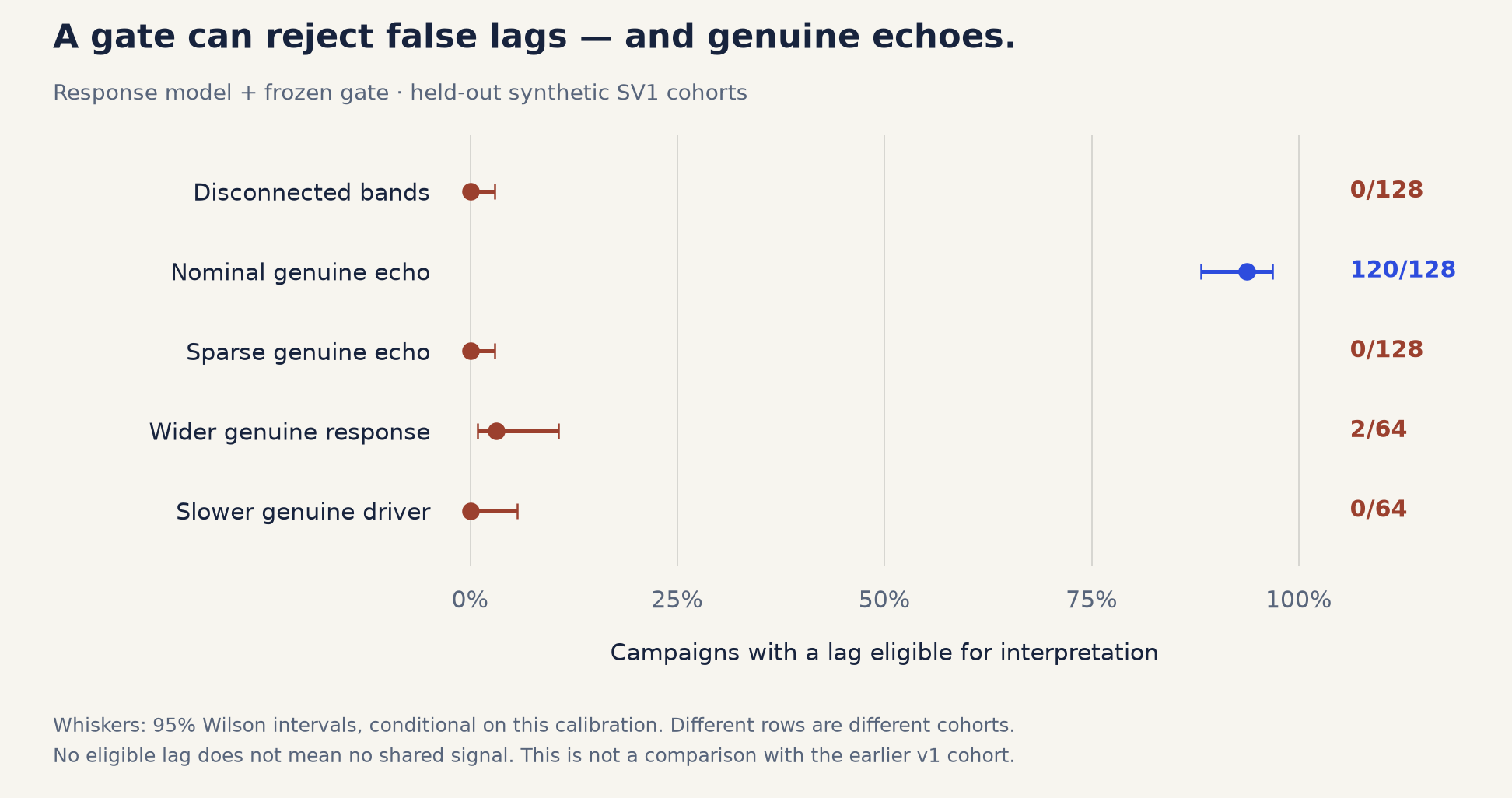
Each row shows how often the response model’s selection rule accepts a delay in a separate group of simulated campaigns. Most genuine echoes are retained with frequent observations. Sparse observations, a wider spread of response times or slower driving variations lead the rule to withhold most or all genuine delays.
The counts are 0/128 for unrelated signals, 120/128 for the default genuine echo, 0/128 for sparse observations, 2/64 for a wider response and 0/64 for slower driving variations. A withheld delay does not mean that the simulated echo is absent.
The figure comes from the second study, labeled SV1. A “lag” is a time delay; the “frozen gate” is the selection rule fixed before evaluation. Bars show 95% Wilson intervals conditional on the fixed calibration set. Different rows use different groups reserved for evaluation, not the earlier study’s campaigns.
Source: Echo Cartographer’s saved signal-validity results and selection-count table.
Technical details and limits
Read the methods, checks and limitations
Methods & checks
The first study compares cross-correlation, which measures how closely brightness changes align after a time shift, with a model of a delayed, smoothed response. It varies observing frequency, noise, campaign length and missing seasons.
In its default condition, all 48 cross-correlation estimates are close to the true delay. Yet only 16/48 reported 90% uncertainty intervals contain it. One competing delay solution leaves 47/48 recoveries classed as usable.
The response model’s intervals contain the true delay in 48/48 cases in that condition. But it also returns tightly constrained positive delays in 47/48 cases where the brightness records are unrelated.
This count describes estimates made before any rule tests whether a connection exists. It is not a calibrated false-positive rate.
The second study uses separate simulated campaigns and adds a selection rule, called a gate. It checks evidence that the signals are connected and whether the response model describes them adequately before accepting a delay for interpretation.
The rule selects existing estimates without repairing their uncertainty intervals. Among this study’s own 128 densely sampled unrelated signal pairs, 127/128 estimates show constrained positive delays before selection and 0/128 are accepted afterwards.
In the second study’s densely sampled genuine-echo tests, the rule accepts 120/128 delays, and 118/120 accepted intervals contain the true delay. The 0/128 false admissions have a conditional 95% Wilson interval of 0–2.9%; observing none does not establish zero risk.
Only this default response-model configuration meets every usefulness criterion specified in the study’s plan.
Changing the observing conditions or simulated response exposes the cost. Sparse observations retain 0/128 genuine delays. A response spread over a wider range of times retains 2/64, losing 62/64; more slowly varying driving light retains 0/64, losing all 64.
The echoes remain present in the simulations even when their delays are withheld.
Code & sources
Public repository containing both simulation studies
Two methods tested across observing conditions
Separate calibration, evaluation and saved results
Accepted measurements and the echoes that were withheld
Saved simulated selection counts and uncertainty intervals